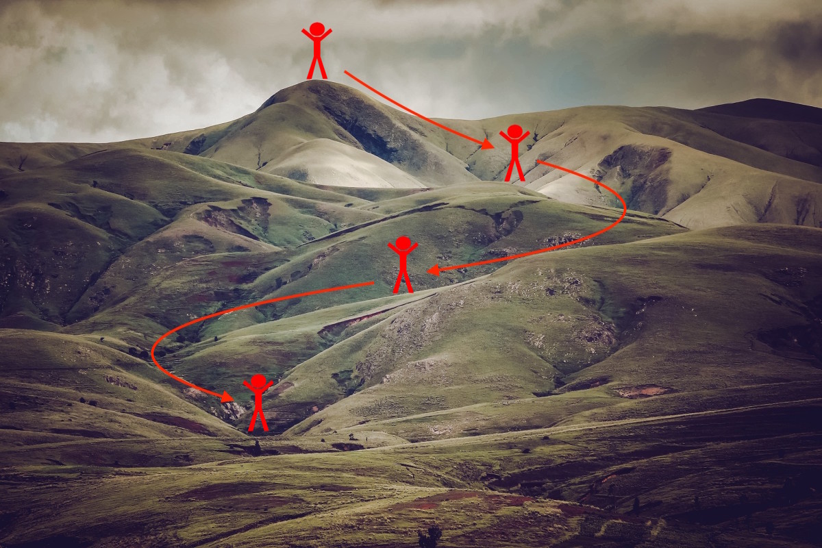
Data Science Enthusiast Gradient is the measure of increase or decrease in the magnitude of a property. Descent indicates a drop in the property. Gradient Descent algorithm, in simple words, can be defined as an algorithm that minimizes a cost function iteratively by modifying its parameters until it finds the local minimum. Before we delve into gradient descent and its working, let us briefly talk about cost function.
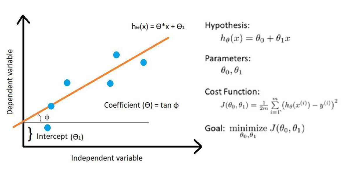
Cost Function
Cost function is a way of determining the accuracy of a model. It measures the separation between actual and predicted values and displays it in the form of a number. In case of regression, the separation between these values should be the minimum which implies that the cost function should be as small as possible.
Working of Gradient Descent
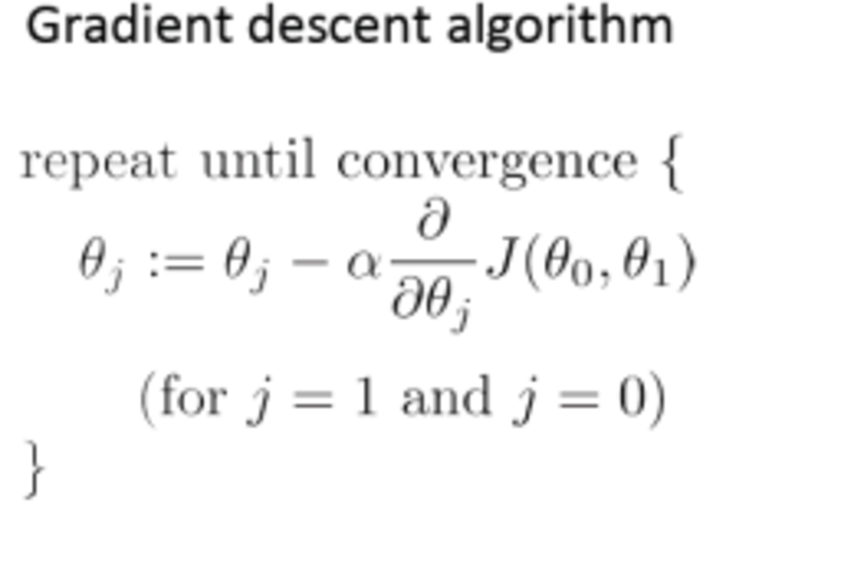
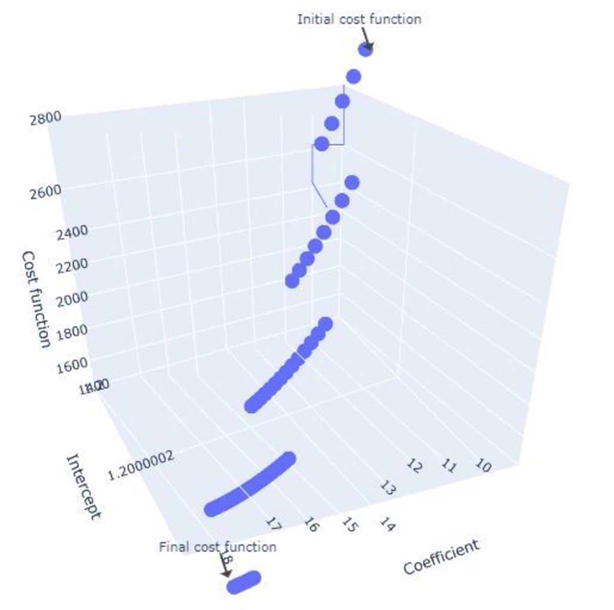
Gradient descent minimizes the cost function by simultaneously updating both parameters, coefficient and intercept, until it finds the local minimum.
1. Modelling Without intercept
In this section, we will implement gradient descent considering only the coefficient (i.e., intercept=0). Code: Result:
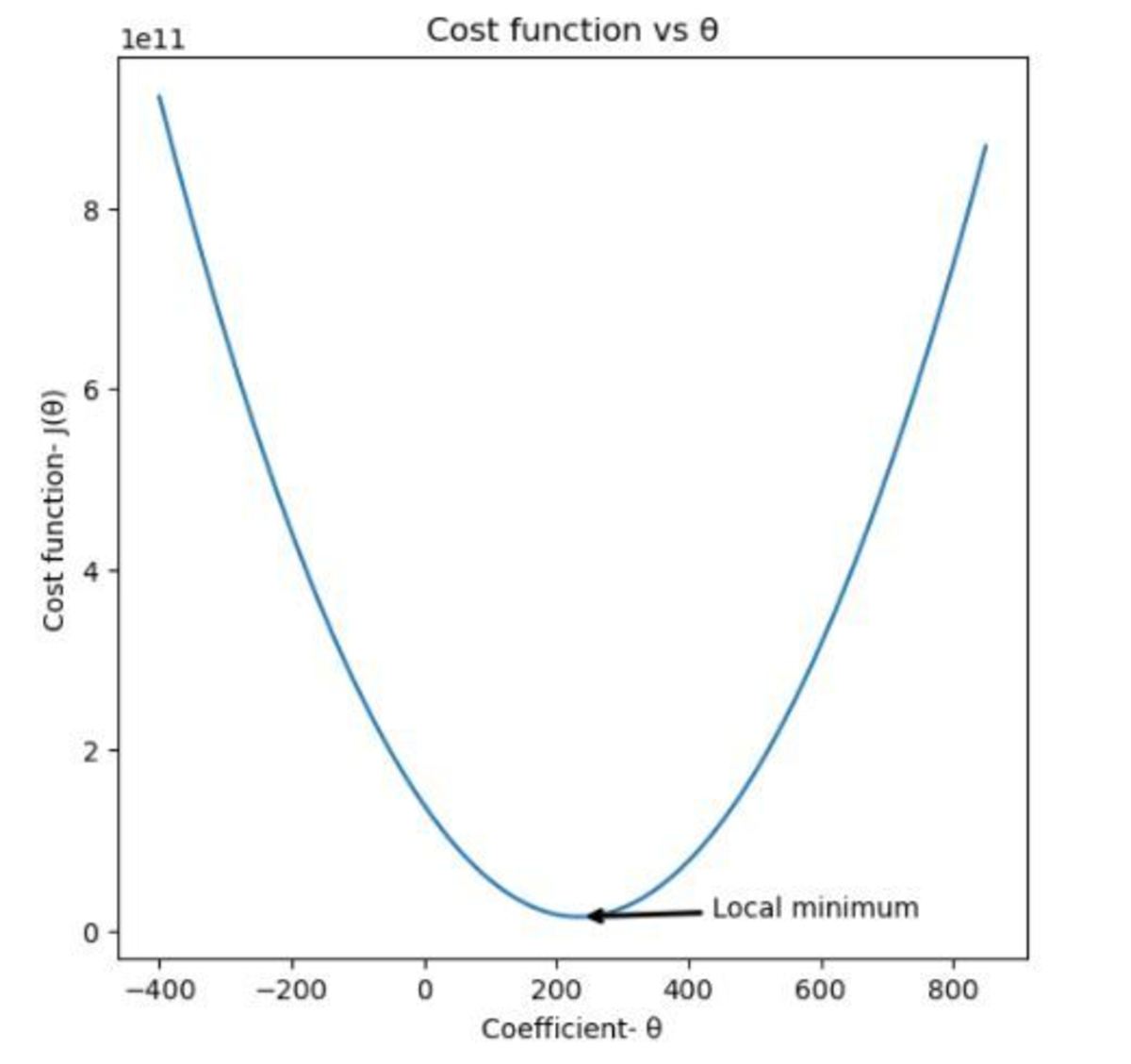
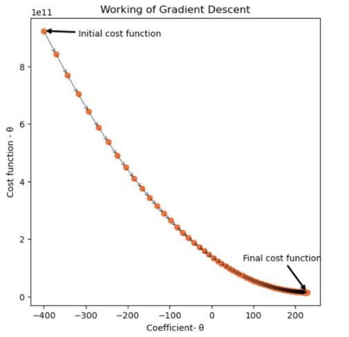
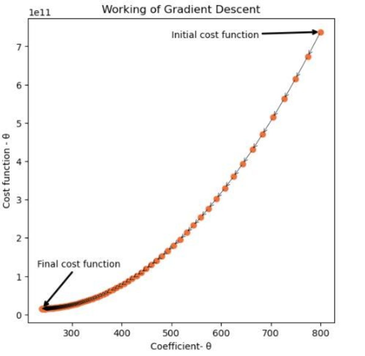
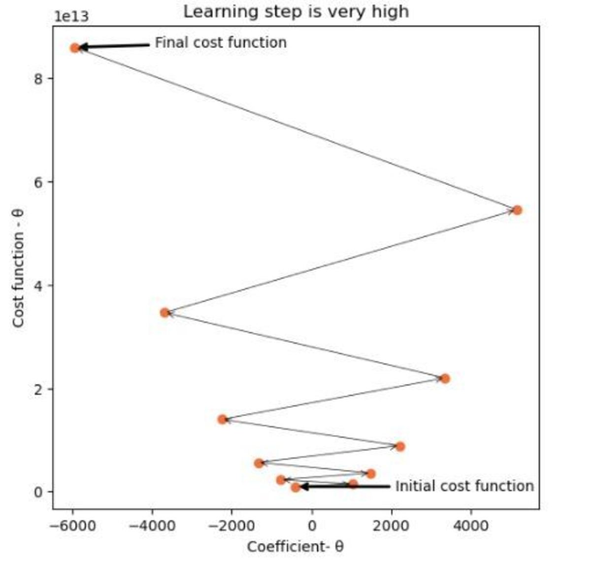
The above chart shows the cost function plotted for a set of coefficients ranging from -400 to 850. It can be observed that the cost function minimizes a certain value of coefficient. Here, gradient descent starts with a coefficient value equal to -400 and works iteratively to bring down the value of cost function over 100 iterations. In this case, gradient descent starts with a value equal to 800 and runs over 100 iterations. Both the cases run on the same value of learning step. How is gradient descent able to work in two different directions? You must be wondering why does it work differently in the above two cases. The above cases clearly show that gradient descent can work in two different directions. In plot 1 it works from left to right while in plot 2 it works from right to left. This is because of the derivative term which is being subtracted from the initial value of the coefficient (Refer to gradient descent algorithm under the Working of Gradient Descent section). This derivative is simply the slope of the curve at any point. In the first case, the slope of the curve is negative, which results in a positive term being added to the coefficient. Hence, the value of coefficient increases in subsequent iterations. In the second case, the slope of the curve is positive, hence the value of coefficient keeps on decreasing. What if the learning step of gradient descent is set too high? For gradient descent to work correctly, it is important that to set the learning step to an appropriate value. Large learning rate means big steps. If the learning step is set too high, the algorithm may never be able to make it to the local minimum as it bounces back and forth between the convex function as in the above scenario. If the learning rate is very small, the algorithm will eventually find the local minimum. However, it may work quite slowly.
2. Modelling With intercept
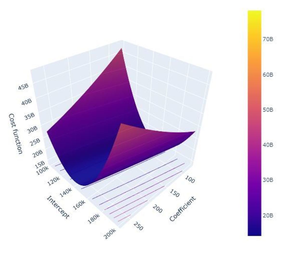
Here, we consider both coefficient and intercept to assume some finite value. Code: Result: In this case, the cost function not only depends on the coefficient, but also on the intercept. The above plot shows the cost function plotted for a range of values of the coefficients and intercepts. Note that the graph contains a global minimum. The above image summarizes the working of gradient descent when both coefficient and intercept participate. It can be clearly seen that both the parameters are updated simultaneously until the cost function reaches its local minimum.
Check your knowledge:
For each question, choose the best answer. The answer key is below.
Answer Key
Interpreting Your Score
If you got 2 correct answers: Well done! This content is accurate and true to the best of the author’s knowledge and is not meant to substitute for formal and individualized advice from a qualified professional. © 2021 Riya Bindra
